Value of Renewable Electricity
Learning objectives
In this chapter, we will learn more about the economics of renewable energy, with a focus on the economic “value” of wind and solar electricity. At the end of the chapter, the reader will be able to:
- Differentiate between short term and long-term drop in value of wind and solar electricity
- Understand that this value drops with penetration
- Discuss various measures to mitigate this value drop
- Know the framework for determining the optimal level of RE in an electricity system
1. Value of wind and solar energy
The economist of anything has two sides: cost and value. To see if and to what extent renewable energy is economic (both from an investor and from society’s point of view), one needs to study its cost. But one also needs to study its value, which we will do now.
1.1. Empirical data
Empirics. Let us start with a look at empirical data. The table below contains electricity price data for Germany for the years 2001 to 2016. The first column shows the average day-ahead electricity price, the so-called “base price”. The base price equals the average income of a “perfect” base load plant that operates all year round. Along with the base price of electricity, the table also contains the market value of wind and solar power as defined in The price and value of electricity. The second and fourth columns show market value (the average income in EUR per MWh) of onshore wind and solar respectively.
| Year | Base price of electricity (1) | Market value of Wind (€/MWh) (2) | Value factor of Wind (3) | Market value of Solar (€/MWh) (4) | Value factor of Solar (5) |
|---|---|---|---|---|---|
| 2001 | 23 | 23 | 1.01 | 27 | 1.19 |
| 2002 | 23 | 22 | 0.98 | 29 | 1.30 |
| 2003 | 29 | 28 | 0.95 | 38 | 1.30 |
| 2004 | 29 | 28 | 0.99 | 34 | 1.19 |
| 2005 | 46 | 44 | 0.96 | 53 | 1.15 |
| 2006 | 51 | 47 | 0.92 | 65 | 1.27 |
| 2007 | 38 | 35 | 0.92 | 43 | 1.13 |
| 2008 | 66 | 62 | 0.94 | 81 | 1.23 |
| 2009 | 39 | 37 | 0.94 | 43 | 1.11 |
| 2010 | 44 | 42 | 0.95 | 49 | 1.09 |
| 2011 | 51 | 47 | 0.92 | 56 | 1.10 |
| 2012 | 43 | 37 | 0.88 | 44 | 1.04 |
| 2013 | 38 | 32 | 0.85 | 37 | 0.98 |
| 2014 | 33 | 28 | 0.86 | 32 | 0.98 |
| 2015 | 32 | 27 | 0.85 | 31 | 0.98 |
| 2016 | 29 | 25 | 0.85 | 27 | 0.93 |
Source: OEE based on load data
Value factor. The above table (third and fifth columns) also shows the “value factor” for each technology, which is the ratio of market value of each technology to the base price of electricity.
\begin{equation} \label{eq:3} LCOE= \frac{\sum_{t=1}^{T} G_t \cdot P_t} {\sum_{t=1}^{T} G_t} / \frac{\sum_{t=1}^{T} P_t} {T} \end{equation}
Where Gt is the electricity generation (in MWh) of wind/ solar plants and Pt the average market price (in EUR/MWh) in time period t.
From boom to bust. From the data in the table, we can see that electricity prices change over the years. During the 2000s prices were on the rise, a consequence of the commodity price boom and strong demand. After 2008 electricity prices followed a downward trend until 2016. This is a long and deep boom-bust cycle that caused a profound crisis of European electricity utilities, a topic to which we return in the chapter on Reasons for the price drop.
Diminishing returns. More importantly, however, it can be observed that the relative price of wind energy – the wind value factor – declined continuously during the entire cycle. Plotted against the share of wind and solar energy in electricity consumption, this pattern becomes more obvious (Figure 1). With increasing penetration the relative value of wind and solar energy has declined. For economists this pattern should not come as a surprise: if the supply of commodity increases, its relative price goes down. The reasons why this pattern was overlooked for many years is the complexity of electricity markets, where prices changes from hour to hour and the fact that renewable power was being paid above-market tariffs (see chapter on Support Schemes).
Figure 1. Wind and solar value factors in Germany 2001-16
Key point: The relative value of wind and solar energy diminishes with increasing market share.
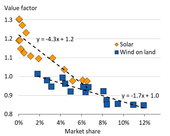
Source: Own work based on data from EPEX Spot, Arbeitsgemeinschaft Energiebilanzen, German TSOs and ENTSO-E. Updated from Hirth (2013)
Notes: Value Factor = Market value / base price. Each symbol represents one year. Extrapolation suggests that at 30% wind share its value factors is 0.5; at 15% solar its value is 0.56.
From high value… At low penetration rates, the value of wind and, in particular, solar energy was above the average electricity price. The reason was that in Germany electricity demand and supply of renewable energy is positively correlated: electricity demand is higher in winter times when winds tend to be stronger (positive seasonal correlation). Similarly, electricity demand is higher around noon when solar irradiance is high (positive diurnal correlation). So renewable energy is high-value electricity!
… to low value. However, as the share of wind and solar power increases in the system, its value declines. We have observed this fact above, but how can we explain it? Here the merit-order model is insightful. Figure 2 compares two cases: the market-clearing price in a given hour without, and with, supply of wind energy. Without wind power in the system the market-clearing price is given by inter-section of the load curve and the merit order curve. When renewables are supplying power to the system, the market-clearing price is given by intersection of the net load curve and merit order curve. Note that the market price decreases when renewables are generating electricity. This is not a coinci-dence: it is the additional supply itself that drives down the price. The reduction in market prices on introduction of renewables in the system is supported by computer models that account for factors like import/ export of power, elastic demand etc.
Cannibalization vs. merit-order effect. This reduction in wind and solar market value has some-times been called a “self-cannibalization effect”. In fact, it is simply the result of extra supply depressing the price. It reflects a general pattern in economics: if there is additional supply of a good (say, wind energy), its relative price declines. Note, however, that the price-depressing effect occurs only when the wind is blowing or the sun is shining. In the next hour, prices may increase again. It can even be shown that for moderate rates renewables penetration, the long-term average price is not affected by additional wind/solar power, but the wind/solar market value declines (Lamont 2008). The reduction of prices during windy/sunny hours should not be confused with a general (temporary) reduction of the electricity price level if large amounts of renewable energy are introduced within few years. This latter phenomenon has been called, somewhat confusingly, the “merit-order effect”.
Figure 2. The merit-order model in a windy hour
Key point: The additional supply of (wind) energy depresses the market-clearing price.
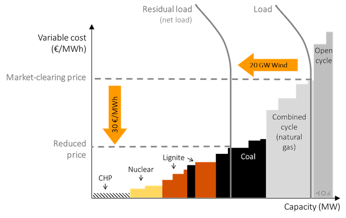
Source: Own work. Updated from Hirth (2013) Notes: Numbers are illustrative, but realistic in size.
Consequences of decline in market value. The loss of market value jeopardizes profitability of renewables investments, the phase-out of support schemes, renewable energy targets and ultimately decarbonization of the power system. It is bad news for investors in renewables and the renewables industry but also tax payers and the climate. To assess how severe the consequences might be we need to know if the decline in market continues as penetration rates increase. Extrapolating historical trends linearly into the future is certainly a bad idea, in particular where highly non-linear systems like power systems are concerned.
1.2. Model Results
Model Results. In Hirth (2013) we have provided such calculations derived from the open source long-term power market EMMA. You can think of EMMA as the screening curve analysis we conducted in Optimal capacity mix and scarcity pricing, just with additional real-word power system complexities such as balancing power, electricity storage and imports and exports. Figure 3 shows the results of that exercise, along with the market data from above. The model shows that under “business-as-usual” assumptions, the market value keeps dropping albeit at a diminishing pace. At a market share of 30%, we might expect a wind value factor of 0.65, down from 0.85 today and above 1 when the first turbine was deployed. In other words, compared to value at the start of wind energy deployment each MWh of wind energy will be worth only 40 percent as much when the share of wind energy increases to 30 percent. This is a pretty significant loss of economic value.
Figure 3. Wind value factor: market data and model results
Key point: Computer models indicate that the value drop of wind energy continues, albeit not linearly.
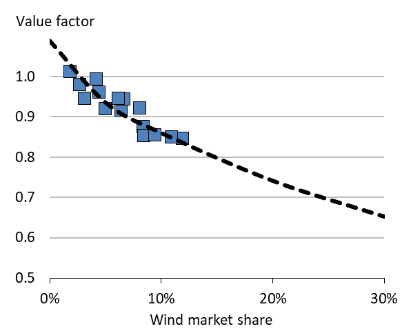
Source: Own work. Updated from Hirth (2013).
The value of solar. The model results depicted by Figure 4 as well as the market data summarized above (Figure 1) indicate that solar energy loses value even quicker than wind energy. The drop for each percentage point in market share is about three times as large, according to these figures. The reason for this difference lies in the different patterns of wind and solar energy production. The output of solar energy is compressed in less hours of the year. This is reflected in capacity factors that are roughly half of wind capacity factors. As a consequence, to reach the same energy market share, about twice the capacity is required. This implies that, when the sun is shining, large amounts of cheap energy are flooding the market and the price drop is particularly pronounced. As a consequence, the market value of solar energy drops faster.
Figure 4. Solar value factor: market data and model results Key point: Computer models indicate that the value of solar energy drops significantly faster than that of wind energy.
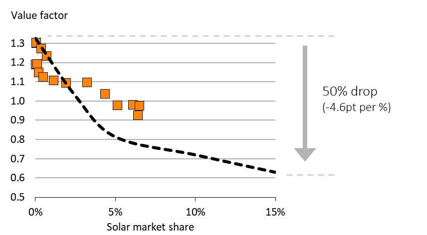
Source: OEE. Updated from Hirth (2013)
Other studies. Few published studies explicitly report the market value of wind energy. However, any study that reports hourly-data of wind generation and electricity prices does so implicitly. Figure 5 shows 18 of such studies, for each of which we translated the raw results into the value factor of wind energy. The studies disagree on the level of the wind value factor, reflecting the diversity of geographies covered as well as the diversity of methods and assumptions. Some studies report a steeper drop than others. However, each study individually as well the body of studies collectively strongly suggest that the value of wind power does drop with the share of wind energy in annual electricity consumption.
Figure 5. Wind value factor: literature review
Key point: Different studies disagree on the level, but they all confirm that the value factor tends to decline with market share.
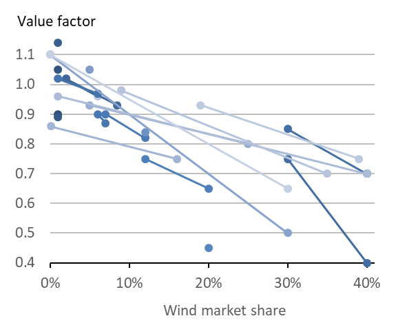
Source: Own work. Updated from Hirth (2013)
Note: Each line represents one study or one scenario, with end points indicating the max/min market shares.
Further reading. Next to the papers cited above (Hirth 2013, Lamont 2008), we recommend Joskow (2011) for an accessible qualitative discussion of the market value of renewable energy and Mills & Wiser (2012, 2014) for model-based estimates. For more data on solar energy, see Hirth (2015).
1.3. Mitigating the value drop
The market value of wind (and solar) energy depends on many factors. From the merit-order model of electricity prices (Figure 2), it is evident that a steeper merit-order curve will tend to increase the value drop for a given expansion of renewable energy. Therefore, anything that makes the merit-order curve flatter will tend to reduce the drop in value. Similarly, a more flexible power system that has significant energy storage, capability to import/export electricity and price-elastic electricity demand will mitigate the value drop.
Storage. What happens if the power system reacts more flexibly to wind supply as was assumed in the model runs? One reason for more flexibility could be a higher amount of energy storage in the system. If additional wind supply depresses the electricity price, storage operators would take this opportunity to fill their tanks, thereby creating additional demand and increasing the prices (com-pared to the no-storage case). In effect, the presence of storage makes electricity demand price-elastic. If unlimited amounts of loss-free storage capacity would be available for free, the result would be an always-flat electricity price. Wind energy would not depress the price and all generation technologies would have the same market value. (The electricity market would also become a very boring type of market and electricity economists would not be needed any more.) A more realistic case, however, is assessing the impact of limited amounts of storage that is subject to losses. Figure 6 presents one such case. Here, the amount of existing pumped hydro storage was, in the first run, set to zero. In the second run, it was fixed at twice the real capacity. The impact is as expected: the addition-al flexibility helps mitigating wind energy’s value drop. However – and that’s a big however –, the impact is relatively small. The take away is that we need to be able to store a lot of energy to make a real difference for the market value of wind energy.
Figure 6. Wind value factor: the impact of energy storage
Key point: Doubling existing storage capacity helps, but only a little.
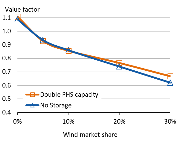
Source: Own work. Updated from Hirth (2013). Notes: PHS is pumped hydro storage. No other type of storage was modelled.
Interconnectors. Many power markets are connected to neighboring markets to be able to import and export electricity. The lines connecting the markets are called interconnectors. In Europe, in particular, many markets are quite well interconnected. Extreme examples include Denmark and Switzerland, which could serve its entire load from imports. More interconnector capacity is mitigating the wind value drop, as wind energy can be exported: the low price during windy times incentivizes additional exports, which increase value of wind (compared to the no-interconnector case). Figure 7 shows that the doubling existing interconnector capacity has a sizeable impact. Still, it can mitigate only a small share of the value drop.
Figure 7. Wind value factor: the impact of interconnectors
Key point: Increasing import/export possibilities helps – but it is not a silver bullet, either.
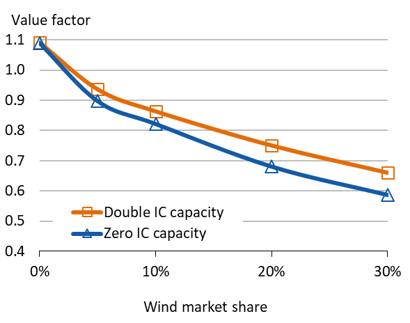
Source: Own work. Updated from Hirth (2013). Note: IC is interconnectors between bidding zones.
Further reading. We regard the drop in wind and solar market value as one of the most critical issues for 21st century power systems. Consequently, several chapters of this book will discuss different options to mitigate the value drop:
- In Optimal capacity mix and scarcity pricing, we have discussed that wind and solar energy are better complemented with low-capex mid load and peaking plants, rather than base load plants. This shift in the technology mix helps mitigating the value drop. (But it is already ac-counted for in the above model results.)
- In System-friendly renewables, we will discuss how low wind-speed turbines increase the market value of wind energy.
- In Heat and electricity, we will discuss possibilities to make electricity demand for heating as well as electricity supply in combined heat and power plants for price responsive, thereby mitigating the value drop.
A number of articles and report assess a range of “mitigation options”, including Hirth (2013, 2015), Hirth & Müller (2016), Mills & Wiser (2012, 2014), and Wiser et al. (2017).
2. Optimal deployment
Back to econ 101. This chapter discussed the generation costs (LCOE) and the market value of renewable energy. Together, these two concepts can be applied in a simple standard economic framework to determine the long-run optimal (or equilibrium) deployment of a certain generation technology, say wind power. The market equilibrium will only coincide with the social optimum, of course, if market are perfect and complete, i.e. they are competitive and all externalities are prices – including carbon emissions.
Long-run marginal costs and benefits. In microeconomics jargon, the LCOE is nothing but the long-run marginal cost and market value is the long-run marginal benefit. Like any other commodity, the equilibrium quantity of the commodity is given by the intersection of the two curves as shown in Figure 8. Here the good concerned is “wind energy”, and it turns out exact the same textbook analysis is feasible, despite peculiar characteristics of the commodity electricity.
Static analysis. Note that this analysis is static in nature, ignoring dynamic changes like learning effects and adaptation of power systems and markets. In a static framework, the long run marginal cost curve (the levelized cost of wind energy) increases with deployment, as the good wind sites are taken first and investors need to progressively move to lower wind speed areas. The long run marginal benefit curve is the market value of wind power. As we have seen, it is downward-sloping. Wind energy should (and will be, in a free electricity market) deployed up to the point where market value and LCOE are identical. If the society aims for a higher share of wind energy in electricity generation, it needs to pay out a price to investors that is higher than the market price, i.e. a subsidy.
Figure 8. Long-term optimal wind deployment
Key point: Optimal deployment levels are determined by the intersection of long-term marginal costs (LCOE) and long-term marginal benefits (market value).

Source: OEE
Cost reductions. Of course the real world is not static. As we have seen in this chapter, the levelized cost of renewable energy have dropped strongly during the past years. This can be depicted in the same graphical framework as a shift of the long-run marginal cost curve to the right. As a consequence, optimal deployment increases.
Figure 9. The impact of cost reduction on optimal wind deployment
Key point: Reducing LCOE will increase optimal deployment.
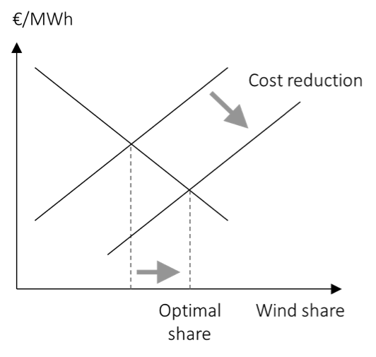
Source: OEE
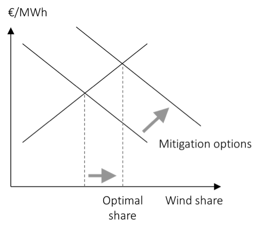
Cost reductions. No only renewable energy cost decline, also power systems adopt to RE deployment. Increasing storage and transmission grid capacity, flexible thermal and hydro power plants, demand response, and smarter markets and system operation will tend to mitigate the drop of wind and solar market value. Deploying system-friendly wind energy will have a similar effect. This can be depicted as a shift of the long-run marginal benefit curve to the right. As a consequence, optimal deployment increases.
Figure 10. The impact of mitigation options on optimal wind deployment
Key point: Mitigating the value drop though increasing power system flexibility or through system-friendly renewables will increase the optimal deployment.
Source: OEE
Further reading. Of course system transformation and RE cost decline happen at the same time. Hirth (2015) presents model-based estimates of optimal deployment of wind and solar energy, using the line of thinking developed here.